4. Systems of linear equations - Mathematics for Business

4.1Introduction¶

When we were learning about the determinant of a matrix, we learned how to solve Cramer’s systems. Cramer’s system is a very special kind of a system because its matrix of coefficients $A$ is invertible. In this chapter, we are going to learn how to solve general systems of linear equations.

First, notice that not all systems of linear equations have a solution.

Therefore, we need to answer to questions:

When does a given system of linear equations have a solution?
If the given system has a solution, how do we compute it?

4.2Kronecker-Capelli theorem¶

The following theorem gives us a way of checking if the given system of linear equations does have or does not have a solution.

4.3Gauss-Jordan method¶

Now that we know how to check whether or not a given system of linear equations has a solution, we want to know how to explicity compute the solutions (if they exist).

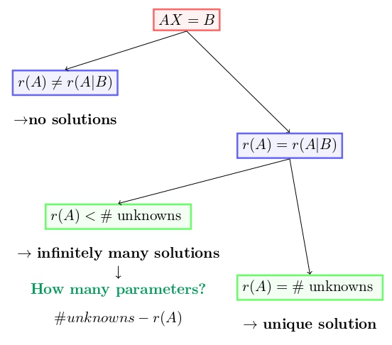
The following diagram tells us the whole story about the number of solutions of a given system of linear equations.

Number of solutions of a system is completely determined by the rank.

4.4Input-output model¶

In this section we are going to use all of the things we learned about matrices and systems of linear equations to study one important economic model called the input-output model. We are going to use it to model a scenario in which we have different sectors of an economy that interact with each other, meaning that every sector consumes outputs of other sectors in order to produce its output. Alongside every sector consuming a part of outputs of all other sectors, each sector has its own demand which is just the amount of output of that sector that is not being used for further production, but rather for export.

The assumptions of the input-output model are:

if the inputs into some sector increase $p$ times, then the output of that sector increases $p$ times as well
the ratio of inputs that a certain sector uses is constant

Note that the first assumption is all about linearity, hence we use linear algebra to study this model.

Throughout this section, we will be using the following notation:

total output of the $i$ -th sector $\dots Q_i$
vector of outputs $\dots Q = \begin{bmatrix} Q_1 & \dots & Q_n\end{bmatrix}^T$
final demand of the $i$ -th sector $\dots q_i$
vector of demands $\dots q = \begin{bmatrix} q_1 & \dots & q_n \end{bmatrix}^T$
intermediate output $\dots Q_{ij}$
technical coefficient $\dots a_{ij}$
matrix of technical coefficients $\dots A = [a_{ij}]$
technology matrix $\dots T = I - A$

We are also going to be using the following formulas of the input-output model:

In order to completely describe the dependencies between the sectors, one needs to calculate all the total outputs $Q_i,$ all the intermediate outputs $Q_{ij}$ and all the final demands $q_i.$ Those values are usually represented using the input-output table:

\begin{array}{c | c | c} Q_i & Q_{ij} & q_i \\ \hline Q_1 & Q_{11} \quad \dots \quad Q_{1n} & q_1 \\ \vdots & \vdots \quad \quad \quad \quad \vdots &\vdots \\ Q_n & Q_{n1} \quad \dots \quad Q_{nn} & q_n \end{array}

Solution to Problem 4.6

The first column of the matrix $A$ denotes the percentages that the outputs of all sectors play in the production of 1 unit of output of the first sector. Therefore, in order to find the intermediate outputs used by the first sector, we need to multiply the first column of the matrix $A$ by $Q_1 = 100.$ We can use the same reasoning to find the intermediate outputs used by the second and the third sector - we multiply the second and the third column of the matrix $A$ by $Q_2$ and $Q_3,$ respectively. Therefore, the input-output table is given by

\begin{array}{c | c | c} Q_i & Q_{ij} & q_i \\ \hline 100 & 20 \quad 30 \quad 10 & 40 \\ 200 & 10 \quad 60 \quad 25 & 105 \\ 100 & 20 \quad 40 \quad 10 & 30 \end{array}

Solution to Problem 4.7

The first sector has increased its output $\frac{110}{100} = 1.1$ times, so the intermediate outputs that are used by the first sector must increase 1.1 times as well. Therefore, to find new intermediate outputs that are being used by the first sector, we need to multiply the old ones by 1.1. In the same way we can find the intermediate outputs used by the second and the third sector. So, the input-output table is given by

\begin{array}{c | c | c} Q_i & Q_{ij} & q_i \\ \hline 110 & 33 \quad 33 \quad 33 & 11 \\ 165 & 33 \quad 22 \quad 66 & 44 \\ 165 & 22 \quad 33 \quad 44 & 66 \end{array}

Solution to Problem 4.8

Remember, the first column of the matrix $[Q_{ij}]$ tells us how many units of all sectors are being used by the first sector in order to produce $Q_1$ units of output. Similarly, the second column of the matrix $[Q_{ij}]$ tells us how many units of all sectors are being used by the second sector in order to produce $Q_2$ units of output. Hence, we can easily find the matrix of technical coefficients:

A = \begin{bmatrix} 1/5 & 1/2 \\ 2/5 & 0 \end{bmatrix}.

Therefore, the technology matrix is given by

T = \begin{bmatrix} 4/5 & -1/2 \\ -2/5 & 1 \end{bmatrix}.

The inverse of the technology matrix is then given by

T^{-1} = \begin{bmatrix} 5/3 & 5/6 \\ 2/3 & 4/3 \end{bmatrix}.

Now we have

Q^{\text{new}} = T^{-1} \cdot q^{\text{new}} = \begin{bmatrix} 250 \\ 160 \end{bmatrix}.

Now we can find the input-output table in the same way as we did in Problem 4.6:

\begin{array}{c | c | c} Q_i & Q_{ij} & q_i \\ \hline 250 & 50 \quad \quad 80 & 120 \\ 160 & 100 \quad \quad 0 & 60 \end{array}

Solution to Problem 4.9

In Problem 4.6 we have seen that it is very easy to find the input-output table if we know the vector of outputs $Q = \begin{bmatrix} Q_1 & Q_2 & Q_3 \end{bmatrix}^T.$ So, we only need to find the total output $Q_2$ of the second sector in order to know what is $Q$ equal to. That output $Q_2$ can be calculated as follows:

\begin{split} Q_2 &= Q_{21} + Q_{22} + Q_{23} + q_2 \\ &= a_{21}Q_1 + a_{22}Q_2 + a_{23}Q_3 + q_2 \\ &= 3 + 0.2Q_2 + 12 + 1 \\ &= 0.2 Q_2 + 16 \end{split}

From this equation is follows that

0.8 Q_2 = 16 \implies Q_2 = 20.

So, $Q = \begin{bmatrix} 10 & 20 & 30 \end{bmatrix}^T$ and we can find the input-output table in the same way as we did in Problem 4.6:

\begin{array}{c | c | c} Q_i & Q_{ij} & q_j \\ \hline 10 & 0 \quad 2 \quad 6 & 2 \\ 20 & 3 \quad 4 \quad 12 & 1 \\ 30 & 2 \quad 6 \quad 3 & 19 \end{array}

Solution to Problem 4.10

Again, as we have seen in Problem 4.6, if we know the vector of outputs $Q$ then it is easy to find the input-output table. Hence, we want to find the total outputs $Q_1$ and $Q_3$ of the first and the third sector. Following the same reasoning as in Problem 4.9, those outputs are given by

\begin{split} Q_1 & = 0.1Q_1 + 0.15Q_2 + 0.2Q_3 + q_1 = 0.1Q_1 + 0.2Q_3 + 140 \\ Q_3 &= 0.2Q_1 + 0.1Q_2 + 0.15Q_3 + q_3 = 0.2Q_1 + 0.15Q_3 + 130 \end{split}

Therefore, we have a system of two equations with two unknowns:

\begin{cases} 0.9Q_1 - 0.2Q_3 = 140 \\ -0.2Q_1 + 0.85Q_3 = 130 \end{cases}

The solution of this system is given by

Q_1 = 200, \quad Q_3 = 200.

Hence, the vector of outputs is given by $Q = \begin{bmatrix}200 & 160 & 200\end{bmatrix}^T$ and from here it easily follows that the input-output table is given by

\begin{array}{c | c | c} Q_i & Q_{ij} & q_i \\ \hline 200 & 20 \quad 24 \quad 40 & 116 \\ 160 & 60 \quad 32 \quad 60 & 8 \\ 200 & 40 \quad 16 \quad 30 & 114 \end{array}

Part 1. Linear algebra

3. Rank of a matrix

Part 2. Functions of one variable

5. Domains and limits of functions