11. Homogeneous functions Faculty of Economics and Business
University of Zagreb
11.1 Homogeneous functions ¶ We say that a function f ( x 1 , … , x n ) f(x_1, \dots, x_n) f ( x 1 , … , x n ) homogeneous
f ( λ x 1 , … , λ x n ) = λ α ⋅ f ( x 1 , … , x n ) , f(\lambda x_1, \dots, \lambda x_n) = \lambda^\alpha \cdot f(x_1, \dots, x_n), f ( λ x 1 , … , λ x n ) = λ α ⋅ f ( x 1 , … , x n ) , where α ∈ R \alpha \in \mathbb{R} α ∈ R degree of homogeneity.
Interpretation 1 % , 1\%, 1% , f f f α % . \alpha \%. α %.
Check whether or not the function f ( x , y ) = x 2 + 2 x y + 3 y 2 \displaystyle f(x,y) = x^2 + 2xy + 3y^2 f ( x , y ) = x 2 + 2 x y + 3 y 2
Check whether or not the function f ( x , y , z ) = 2 x ⋅ ln ( z y ) \displaystyle f(x,y,z) = 2x \cdot \ln\left(\frac{z}{y}\right) f ( x , y , z ) = 2 x ⋅ ln ( y z )
The Cobb-Douglas production function is given as
Q ( L , K ) = c L a K b , Q(L,K) = c L^a K^b, Q ( L , K ) = c L a K b , where a , b , c a,b,c a , b , c
Let the Cobb-Douglas function be given as
Q ( L , K ) = 0.2 L 0.3 K 0.6 . Q(L,K) = 0.2 L^{0.3} K^{0.6}. Q ( L , K ) = 0.2 L 0.3 K 0.6 . If both variables L , K L,K L , K 5 % , 5\%, 5% , Q Q Q
Let f ( x , y ) = x ⋅ x 4 + 5 x 2 y 2 + 4 y 4 2 x + y 3 . \displaystyle f(x,y) = x \cdot \sqrt[3]{\frac{x^4 + 5x^2y^2+4y^4}{2x+y}}. f ( x , y ) = x ⋅ 3 2 x + y x 4 + 5 x 2 y 2 + 4 y 4 . f f f x , y x,y x , y 7 % ? 7\%? 7% ?
11.2 Partial elasticities ¶ Let f ( x , y ) f(x,y) f ( x , y ) Partial elasticity of the function f with respect to the variable x
E f , x = x f ⋅ f x . E_{f,x} = \frac{x}{f} \cdot f_x. E f , x = f x ⋅ f x . Analogously, partial elasticity of the function f with respect to the variable y
E f , y = y f ⋅ f y . E_{f,y} = \frac{y}{f} \cdot f_y. E f , y = f y ⋅ f y . Interpretation x x x 1 % 1\% 1% y y y f f f ∣ E f , x ∣ % . \lvert E_{f,x} \rvert \%. ∣ E f , x ∣ %.
As we’ll see in the following problems, partial elasticities have an important economic application.
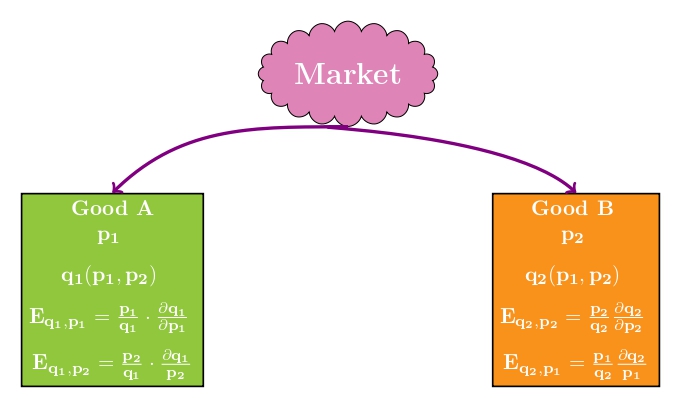
The market with two goods, where each one of them has its own price, demand and elasticity.
We will be refering to the elasticities E q 1 , p 2 E_{q_1, p_2} E q 1 , p 2 E q 2 , p 1 E_{q_2, p_1} E q 2 , p 1 cross-price elasticities, E q 1 , p 1 E_{q_1, p_1} E q 1 , p 1 E q 2 , p 2 E_{q_2, p_2} E q 2 , p 2 price elasticities,
Based on the value of the cross-price elasticities, we have the following categorization of goods on a market:
if E q 2 , p 1 > 0 , \displaystyle E_{q_2, p_1} > 0, E q 2 , p 1 > 0 , substitutes
if E q 2 , p 1 < 0 , E_{q_2, p_1} < 0, E q 2 , p 1 < 0 , complements
There are two goods A A A B B B p 1 , p 2 p_1, p_2 p 1 , p 2
q ( p 1 , p 2 ) = 1 2 p 1 2 + 5 p 2 . q(p_1, p_2) = \frac{1}{2}p_1^2 + \frac{5}{p_2}. q ( p 1 , p 2 ) = 2 1 p 1 2 + p 2 5 . Find the coefficients of price and cross-price elastiticities at p 1 = 1 , p 2 = 2. p_1 = 1, p_2 = 2. p 1 = 1 , p 2 = 2.
11.3 Euler’s Theorem ¶ In this section, we are going to see what is the relationship between homogeneous functions and partial elasticities.
Let f ( x 1 , … , x n ) f(x_1, \dots, x_n) f ( x 1 , … , x n ) f f f α , \alpha, α ,
x 1 f x 1 + ⋯ + x n f x n = α f . x_1 f_{x_1} + \dots + x_n f_{x_n} = \alpha f. x 1 f x 1 + ⋯ + x n f x n = α f . Notice that the equation in Euler’s Theorem
E f , x 1 + ⋯ + E f , x n = α . E_{f, x_1} + \dots + E_{f,x_n} = \alpha. E f , x 1 + ⋯ + E f , x n = α . Let f ( x , y ) = y 3 x 2 ln ( x ( y − x ) y 2 ) . \displaystyle f(x,y) = \frac{y^3}{x^2} \ln \left(\frac{x(y-x)}{y^2}\right). f ( x , y ) = x 2 y 3 ln ( y 2 x ( y − x ) ) . x f x + y f y . \displaystyle x f_x + y f_y. x f x + y f y .